Case study - Germany • hydrographr

Introduction

Load required libraries

library(hydrographr)
library(rgbif)
library(data.table)
library(dplyr)
library(terra)
library(tools)
library(stringr)
library(leaflet)
library(leafem)
library(sf)
library(tidyr)

Define working directory

# Define the "data_germany" directory, where you have downloaded all the data,
# as the working directory
wdir <- "my/working/directory/data_germany"
setwd(wdir)

# Create a new folder in the working directory to store all the data
dir.create("data")

Species data

We first download the occurrence data with coordinates from GBIF

# Once: Download species occurrence data based on the key of the dataset
# and write out to working directory
spdata_all <- occ_download_get(key="0004551-231002084531237",
                              overwrite = TRUE) %>%
  occ_download_import
fwrite(spdata_all, paste0(wdir, "/data/fish_germany_gbif.csv"),
    row.names = F, quote = F, sep = "\t")

# Import and clean the data
spdata <- fread(paste0(wdir, "/data/fish_germany_gbif.csv"), sep = "\t") %>%
  select(gbifID, decimalLongitude, decimalLatitude, species, year) %>%
  rename("longitude" = "decimalLongitude",
         "latitude" = "decimalLatitude")

head(spdata)

gbifID	longitude	latitude	species	year
4058501303	13.2284	52.5709	Abramis brama	2007
4058501307	13.1564	52.4147	Abramis brama	2007
4058460309	13.1861	52.4576	Abramis brama	2007
4058501314	13.1093	52.4079	Abramis brama	2008
4058501316	13.5746	52.5091	Abramis brama	2008
4058460317	13.1177	52.4017	Abramis brama	2008

Let’s visualise the species occurrences on the map

Let’s define the extent (bounding box) of the study area (xmin, ymin, xmax, ymax)

# Define the extent
bbox <- c(min(spdata$longitude), min(spdata$latitude),
          max(spdata$longitude), max(spdata$latitude))

# Define color palette for the different years of record
factpal <- colorFactor(hcl.colors(unique(spdata$year)), spdata$year)

# Create leaflet plot
spdata_plot <- leaflet(spdata) %>%
  addProviderTiles('Esri.WorldShadedRelief') %>%
  setMaxBounds(bbox[1], bbox[2], bbox[3], bbox[4]) %>%
  addCircles(lng = ~longitude, lat = ~ latitude, 
             color =  ~factpal(as.factor(year)),
             opacity = 1) %>%
  addLegend(pal = factpal, values = ~as.factor(year),
            title = "Year of record")
spdata_plot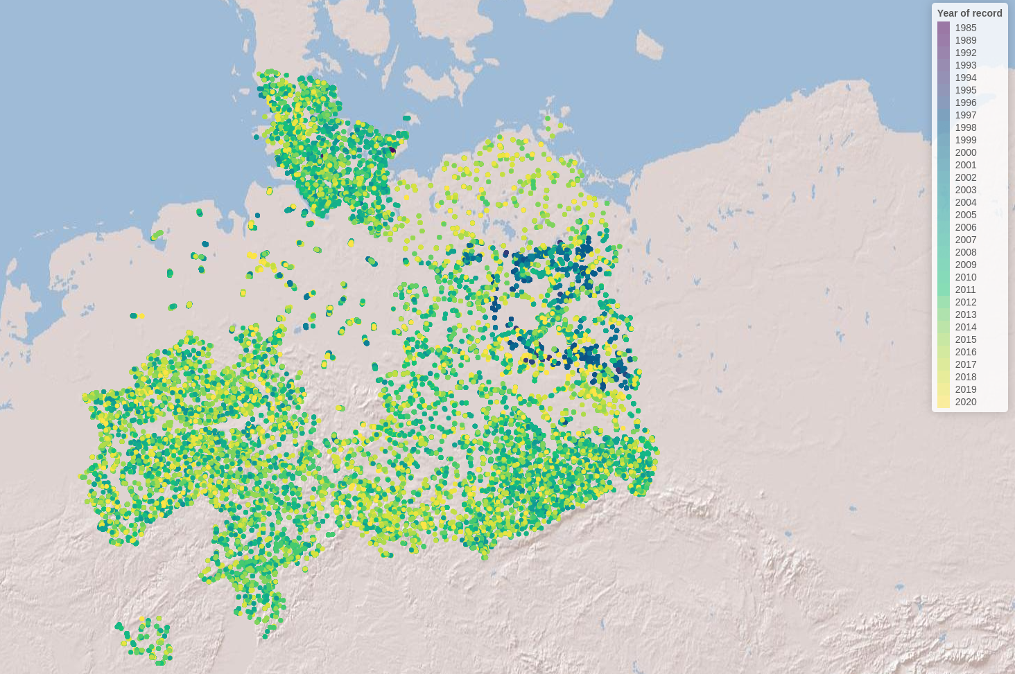

Abiotic variables data

1. Hydrography90m

In order to download layers of the Hydrography90m, we need to know the IDs of the 20°x20° tiles in which they are located. We can obtain these IDs using the function get_tile_id(). This function downloads and uses the auxiliary raster file that contains all the regional units globally, and thus requires an active internet connection.

tile_id <- get_tile_id(data = spdata,
                     lon = "longitude", lat = "latitude")

# Get reg unit id to crop all the regular tile layers so that 
# we have uninterrupted basins
reg_unit_id <- get_regional_unit_id(data = spdata,
                                  lon = "longitude", lat = "latitude")

tile_id

## [1] "h16v02" "h18v00" "h18v02"

Currently the function returns all the tiles of the regional unit where the input points are located. However, some of them may be far from the study area and hence not always needed in further steps. Please double check which tile IDs are relevant for your purpose using the Tile map found here.

In our case, Germany spreads in just one tile, with the ID “h18v02”, so we will keep only this one.

tile_id <- "h18v02"

Then we define the names of the raster and vector layers we want to download.

# Define the raster layers
vars_tif <- c("basin", "sub_catchment", "segment", "accumulation", "direction",
              "outlet_dist_dw_basin", "outlet_dist_dw_scatch",
              "channel_dist_up_seg", "order_strahler")
# Define the vector layers
# The "basin" layer contains the polygons of the drainage basins while the
# "order_vect_segment" layer is the stream network vector file
vars_gpkg <- c("basin", "order_vect_segment")

# Extend timeout to 1000s to allow uninterrupted downloading
options(timeout = 1000)
# Download the .tif tiles of the desired variables
download_tiles(variable = vars_tif, tile_id = tile_id, file_format = "tif",
               download_dir = "data")

# Download the .gpkg tiles of the desired variables
download_tiles(variable = vars_gpkg, tile_id = tile_id, file_format = "gpkg",
               download_dir = "data")

# Download the raster mask of the regional unit
download_tiles(variable = "regional_unit",
               file_format = "tif",
               reg_unit_id = reg_unit_id,
               download_dir = "data")

2. Elevation - MERIT-HYDRO

To download the elevation files of MERIT-HYDRO, we visit https://hydro.iis.u-tokyo.ac.jp/~yamadai/MERIT_Hydro/ to define the tiles that need to be downloaded. We download the zipped tiles into a new directory called elv, unzip the downloaded .tar file and keep only the tiles that we need

elv_dir <- paste0(wdir, "/data/elv") 
dir.create(elv_dir)

3. Climate - CHELSA Bioclim

Finally, we will download three CHELSA present Bioclim variables. For a quick outlook on the bioclimatic variables you can have a look here.

# Create download directory
dir.create(paste0(wdir, "/data/chelsa_bioclim"))

# Extend timeout to 1000s to allow uninterrupted downloading
options(timeout = 1000)

# Download
# Present, 1981-2010
download.file("https://os.zhdk.cloud.switch.ch/envicloud/chelsa/chelsa_V2/GLOBAL/climatologies/1981-2010/bio/CHELSA_bio12_1981-2010_V.2.1.tif",
destfile = "data/chelsa_bioclim/bio12_1981-2010.tif", mode = "wb")
download.file("https://os.zhdk.cloud.switch.ch/envicloud/chelsa/chelsa_V2/GLOBAL/climatologies/1981-2010/bio/CHELSA_bio15_1981-2010_V.2.1.tif",
destfile = "data/chelsa_bioclim/bio15_1981-2010.tif", mode = "wb")
download.file("https://os.zhdk.cloud.switch.ch/envicloud/chelsa/chelsa_V2/GLOBAL/climatologies/1981-2010/bio/CHELSA_bio1_1981-2010_V.2.1.tif",
destfile = "data/chelsa_bioclim/bio1_1981-2010.tif", mode = "wb")

Cropping the raster files

After having downloaded all the layers, we need to crop them to the extent of our study area extended by 500 km, so that our basins are not split in half.

Let’s define the extent (bounding box) of the study area (xmin, ymin, xmax, ymax)

bb <- c(0.256, 20, 45, 55.4325)

We then crop the raster tiles to the extent using the function crop_to_extent() in a loop

for(itile in raster_tiles) {

  crop_to_extent(raster_layer = itile,
                 bounding_box = bb,
                 out_dir = study_area_dir,
                 file_name =  paste0(str_remove(basename(itile), ".tif"),
                                     "_crop.tif"),
                 quiet = FALSE,
                 compression = "high",
                 bigtiff = TRUE,
                 read = FALSE)
}

Filtering the sub-catchment and basin .gpkg files

In case you don’t work on a server, we suggest you to download the output files of this chunk from the following links and then copy them in the folder study_area_dir:

# !! Only run this chunk on a machine with more than 16 GB RAM, 
# as the input files are really big !!

# Load the cropped stream and basin raster layer of the study area.
# The stream raster can be used interchangeably with the sub_catchment raster, 
# because the stream IDs are the same as the sub-catchment IDs. 
# Here we use the stream raster because it's smaller in size. 

stream_layer <- rast(paste0(study_area_dir, "/segment_h18v02_crop.tif"))
basin_layer <- rast(paste0(study_area_dir, "/basin_h18v02_crop.tif"))

# Get all sub-catchment and basin IDs of the study area
subc_ids <- terra::unique(stream_layer)
basin_ids <- terra::unique(basin_layer)

# Get the full path of the stream order segment GeoPackage tile
order_tile <- list.files(wdir, pattern = "order.+_h[v0-8]+.gpkg$",
                         full.names = TRUE, recursive = TRUE)
basin_gpkg_tile <- list.files(wdir, pattern = "bas.+_h[v0-8]+.gpkg$",
                              full.names = TRUE, recursive = TRUE)

# Filter the sub-catchment IDs from the GeoPackage of the order_vector_segment
# tiles (sub-catchment ID = stream ID)
# Save the stream segments of the study area
filtered_stream <- read_geopackage(order_tile,
                                 import_as = "sf",
                                 subc_id = subc_ids$segment_h18v02_crop,
                                 name = "stream")

sf::write_sf(filtered_stream, paste(study_area_dir,
                              paste0(str_remove(basename(order_tile), ".gpkg"),
                                         "_crop.gpkg"), sep="/"))

filtered_bas <- read_geopackage(basin_gpkg_tile,
                                 import_as = "sf",
                                 subc_id = basin_ids$basin_h18v02_crop,
                                 name = "ID")

sf::write_sf(filtered_bas, paste(study_area_dir,
                          paste0(str_remove(basename(basin_gpkg_tile), ".gpkg"),
                                         "_crop.gpkg"), sep="/"))

Merging the elevation tiles

# These are the elevation tiles that include our study area
elv_tiles <- c("n45e000_elv.tif", "n50e010_elv.tif", "n60e000_elv.tif",
                "n45e005_elv.tif", "n50e015_elv.tif", "n60e005_elv.tif",
                "n45e010_elv.tif", "n55e000_elv.tif", "n60e010_elv.tif",
                "n45e015_elv.tif", "n55e005_elv.tif", "n60e015_elv.tif",
                "n50e000_elv.tif", "n55e010_elv.tif", "n50e005_elv.tif",
                "n55e015_elv.tif")

merge_tiles(tile_dir = elv_dir, 
            tile_names = elv_tiles,
            out_dir = study_area_dir, 
            file_name = "elv_study_area.tif",
            compression = "high",
            bigtiff = TRUE,
            quiet = FALSE)


# crop to our extent
crop_to_extent(raster_layer = paste0(study_area_dir, "/elv_study_area.tif"),
               bounding_box = bb,
               out_dir = study_area_dir,
               file_name =  "elv_study_area_crop.tif",
               quiet = FALSE,
               compression = "high", 
               bigtiff = TRUE, 
               read = FALSE)

Finally, we will crop the CHELSA Bioclim layers.

We define the directory containing the layers to be cropped and we list their file names

dir_chelsa <- paste0(wdir, "/data/chelsa_bioclim")
files_chelsa <- list.files(dir_chelsa, pattern = ".tif", full.names = TRUE)

for(ifile in files_chelsa) {
    crop_to_extent(
      raster_layer = ifile,
      bounding_box = bb,
      out_dir = study_area_dir,
      file_name = basename(ifile),
      read = FALSE,
      quiet = TRUE)
}

Extracting sub-catchment IDs

Extract the IDs of the sub-catchments where the points are located. This step is crucial, as many of the functions that we will later use require a vector of sub-catchment IDs as input. Note that the function extract_ids() can be used to extract the values at specific points of any raster file provided to the argument subc_layer. It can be safely used to query very large raster files, as these are not loaded into R.

spdata_ids <- extract_ids(data = spdata,
  id = "gbifID",
  lon = "longitude", lat = "latitude",
  basin_layer = paste0(study_area_dir, "/basin_h18v02_crop.tif"),
  subc_layer = paste0(study_area_dir, "/sub_catchment_h18v02_crop.tif"))

The species data have now their corresponding sub-catchment ids
longitude	latitude	gbifID	subcatchment_id	basin_id
13.2284	52.5709	4058501303	507197109	1294020
13.1564	52.4147	4058501307	507313477	1294020
13.1861	52.4576	4058460309	507278293	1294020
13.1093	52.4079	4058501314	507316793	1294020
13.5746	52.5091	4058501316	507243022	1294020
13.1177	52.4017	4058460317	507321279	1294020

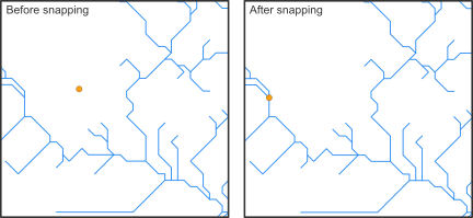
Snapping points to the network

Before we can calculate the distance along the stream network between species occurrences, we need to snap the coordinates of the sites to the stream network. Recorded coordinates of point locations usually do not exactly overlap with the digital stream network and, therefore, need to be slightly corrected.

The hydrographr package offers two different snapping functions, snap_to_network and snap_to_subc_segment. The first function uses a defined distance radius and a flow accumulation threshold, while the second function snaps the point to the stream segment of the sub-catchment the point was originally located in.

For this case study we will use the function snap_to_network to be able to define a certain flow accumulation threshold and ensure that the fish occurrences will not be snapped to a headwater stream (first order stream) if there is also a higher order stream next to it.

# Define full paths of raster layers
stream_rast <- paste0(study_area_dir, "/segment_h18v02_crop.tif")
flow_rast <- paste0(study_area_dir, "/accumulation_h18v02_crop.tif")

# We need to shorten the gbifIDs because they are too long for GRASS-GIS
# We will delete the first 2 characters ("40") from all IDs
spdata_ids$gbifID_tmp <- str_replace(spdata_ids$gbifID, "40", "")

The function is implemented in a for-loop that starts searching for streams with a very high flow accumulation of 400,000 km² in a very short distance and then slowly decreases the flow accumulation to 100 km². If there are still sites left which were not snapped to a stream segment, the distance will increase from 10 up to 30 cells.

# Define thresholds for the flow accumulation of the stream segment, where
# the point location should be snapped to
accu_threshold <- c(400000, 300000, 100000, 50000, 10000, 5000, 1000, 500, 100) 
# Define the distance radius
dist_radius <- c(10, 20, 30)

# Create a temporary data.table
point_locations_tmp <- spdata_ids

# Note: The for loop takes about 9 minutes
first <- TRUE
for (idist in dist_radius) {
    
   # If the distance increases to 20 cells only a flow accumulation of 100 km²
   # will be used
   if (idist == 20) {
    # Set accu_threshold to 100
    accu_threshold <- c(100)
   }
  

  for (iaccu in accu_threshold) {
    # Snap point locations to the stream network
    point_locations_snapped_tmp <- snap_to_network(data = point_locations_tmp,
                                    id = "gbifID",
                                    lon = "longitude", lat = "latitude",
                                    stream_layer = stream_rast,
                                    accu_layer = flow_rast,
                                    method = "accumulation",
                                    distance = idist,
                                    accumulation = iaccu,
                                    quiet = FALSE)

    
    # Keep point location with NAs for the next loop
    point_locations_tmp <- point_locations_snapped_tmp %>% 
      filter(is.na(subc_id_snap_accu))
  
  if (first == TRUE) {
    # Keep the point locations with the new coordinates and remove rows with NA
    point_locations_snapped <- point_locations_snapped_tmp %>% 
    filter(!is.na(subc_id_snap_accu))
    first <- FALSE
  } else {
    # Bind the new data.frame to the data.frame of the loop before
    # and remove the NA
    point_locations_snapped <- point_locations_snapped %>% 
      bind_rows(point_locations_snapped_tmp) %>% 
      filter(!is.na(subc_id_snap_accu))
    
  }
  
  }
    
}

We can write out the result of the snapping

fwrite(point_locations_snapped, paste0(wdir, "/data/spdata_snapped.csv"), sep = ",", 
                      row.names = FALSE, quote = FALSE)

head(point_locations_snapped)

The species data have been attributed new coordinates and in some cases a new sub-catchment id (“subc_id_snap_accu”)
gbifID	longitude	latitude	lon_snap_accu	lat_snap_accu	subc_id_snap_accu
58452301	10.1725	53.8729	10.172083	53.87292	506457237
58452302	10.2972	53.6788	10.297083	53.67875	506528521
58452303	9.4411	54.0136	9.441250	54.01375	506407992
58452304	9.5619	54.0996	9.562083	54.09958	506383004
58452305	10.6518	53.6034	10.652083	53.60375	506562036
58452306	9.9609	53.8553	9.961250	53.85542	506463635

Calculating distances between points

We will calculate the distance between all point locations. The following chunks are computationally heavy, so we suggest to run them on a server.

# Load as graph
stream_graph <- read_geopackage(
  gpkg = paste0(study_area_dir, "/order_vect_segment_h18v02_crop.gpkg"),
  import_as = "graph")

# Get the network distance (in meters) between all input pairs.
# We provide the subcatchment ids of the snapped points to the argument "subc_id"
subc_distances <- get_distance_graph(stream_graph,
                            subc_id = point_locations_snapped$subc_id_snap_accu,
                            variable = "length",
                            distance_m = TRUE)

head(subc_distances)

from	to	distance
506457237	506528521	167973.69
506457237	506407992	92908.34
506528521	506407992	111478.74
506457237	506383004	161571.37
506528521	506383004	136308.05
506407992	506383004	105076.42

Obtaining network centrality indices

We will now calculate centrality indices using the directed stream network graph and the function get_centrality We want to consider only the upstream connected segments, so we set mode = "in".

The following chunks are computationally heavy, so we suggest to run them on a server.

centrality <- get_centrality(stream_graph, index = "all", mode = "in")

We can reclassify the stream segment and sub-catchment raster layers based on the centrality value of each stream, using the function reclass_raster. Essentially, we will create two new raster files, in which each stream pixel will have a centrality value, instead of the unique ID of the stream or sub-catchment.

# This data.frame includes some NAs in some of the columns, because some centrality metrics by default cannot be defined for some the subcatchments. We have to discard subcatchments with NAs before reclassifying.
centrality <- drop_na(centrality)

# Then we convert the values in the centrality data.frame into integers
centrality <- centrality %>% mutate_if(is.numeric, as.integer)

reclass_raster(data = centrality, 
                            rast_val = "subc_id", 
                            new_val = "betweeness", 
                            raster_layer = paste0(study_area_dir, "/segment_h18v02_crop.tif"), 
                            recl_layer = paste0(study_area_dir,"/segment_h18v02_betweeness_all.tif"), 
                            read = F)

reclass_raster(data = centrality, 
               rast_val = "subc_id", 
               new_val = "degree", 
               raster_layer = paste0(study_area_dir, "/sub_catchment_h18v02_crop.tif"),
               recl_layer = paste0(study_area_dir,"/sub_catchment_h18v02_degree_all.tif"), 
               read = F)

reclass_raster(data = centrality, 
               rast_val = "subc_id", 
               new_val = "betweeness", 
               raster_layer = paste0(study_area_dir, "/sub_catchment_h18v02_crop.tif"),
               recl_layer = paste0(study_area_dir,"/sub_catchment_h18v02_betweeness_all.tif"), 
               read = F)

reclass_raster(data = centrality, rast_val = "subc_id", 
               new_val = "farness", 
               raster_layer = paste0(study_area_dir, "/sub_catchment_h18v02_crop.tif"),
               recl_layer = paste0(study_area_dir,"/sub_catchment_h18v02_farness_all.tif"), 
               read = F)

reclass_raster(data = centrality, 
               rast_val = "subc_id", 
               new_val = "eccentricity", 
               raster_layer = paste0(study_area_dir, "/sub_catchment_h18v02_crop.tif"),
               recl_layer = paste0(study_area_dir,"/sub_catchment_h18v02_eccentricity_all.tif"), 
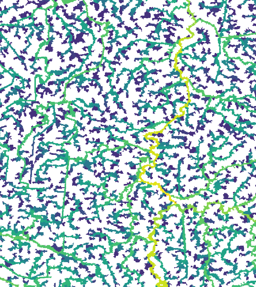
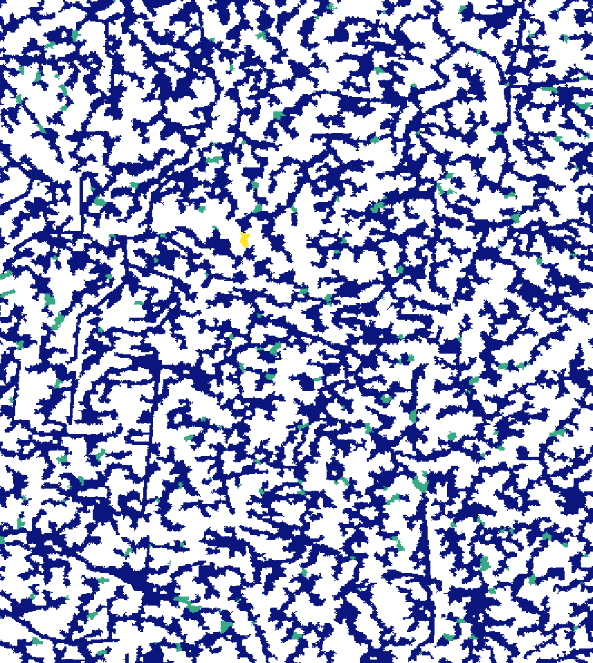
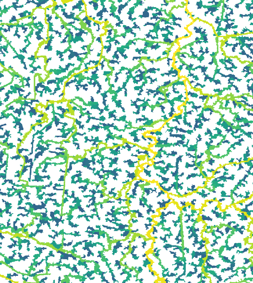
               read = F)

Here’s what the new segment and sub-catchment layers look like on QGIS. Yellow sub-catchments have the highest values, whereas dark blue have the lowest values for the different metrics.

The node betweenness is (roughly) defined by the number of geodesics (shortest paths) going through a node:

The degree of a node is the number of its adjacent edges:

Farness centrality is the sum of the length of the shortest paths between the node and all other nodes. It is the reciprocal of closeness (Altermatt, 2013):

The eccentricity of a node is its shortest path distance from the farthest other node in the graph (West, 1996):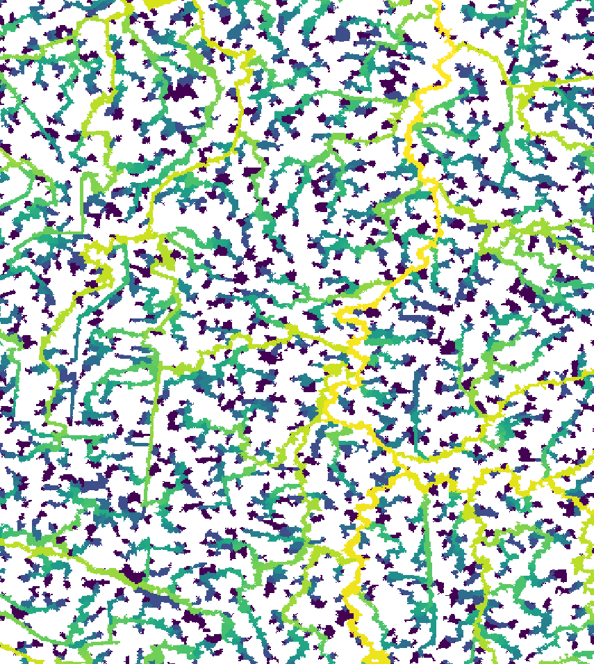

We can add the centrality metrics’ values to the table of our points, using the sub-catchment id:

point_locations_snapped <- left_join(point_locations_snapped, centrality, 
                          by = c('subc_id_snap_accu'= 'subc_id'))
head(point_locations_snapped)

subc_id	degree	closeness	farness	betweeness	eccentricity
506226492	2	4.8e-06	210084	175492	163
506226723	2	3.8e-06	263544	125205	185
506226977	2	1.4e-06	716085	167992	214
506227065	2	3.6e-06	279270	114210	191
506227782	2	6.1e-06	164017	201756	144
506227869	2	7.5e-06	133336	168399	137

Bonus! If we want to include the centrality indices to the stream network .gpkg, we can import the .gpkg and merge it with the centrality table

# Load stream network .gpkg as vector
stream_vect <- read_geopackage(paste0(study_area_dir, "/order_vect_segment_h18v02_crop.gpkg"),
                               import_as = "SpatVect")

# Merge the centrality table with the vector
stream_vect <- terra::merge(stream_vect, spdata_centr, 
                        by.x = c('stream'), by.y="subc_id")

# Write out the stream gpkg including the centrality indices
writeVector(stream_vect, paste0(study_area_dir, "/order_vect_segment_centr.gpkg"))

Extracting zonal statistics of topographic variables

We will calculate the zonal statistics of the Hydrography90m, MERIT-HYDRO DEM and the CHELSA Bioclim variables for the sub-catchments of our species points. Caution, don’t increase the number of cores to more than 3 as this can cause memory problems. However, this highly depends to the number of sub-catchments as well. We recommend to test the function with different parameters to find out what works best for your case.

Let’s first define the input var_layers for the extract_zonal_stat function

list.files(study_area_dir)
var_layers <- c("bio1_1981-2010.tif", "bio12_1981-2010.tif",
                "bio15_1981-2010.tif", "elv_study_area_crop.tif",
                "outlet_dist_dw_basin_h18v02_crop.tif")

A good practice before aggregating the variables is to check their NoData values:

report_no_data(data_dir = study_area_dir, var_layer = var_layers)

#                                 Raster                  NoData
# 1                   bio1_1981-2010.tif                  -99999
# 2                  bio15_1981-2010.tif 3.40282346600000016e+38
# 3 outlet_dist_dw_basin_h18v02_crop.tif                   -9999
# 4                  bio12_1981-2010.tif                  -99999
# 5              elv_study_area_crop.tif                   -9999

# Run the function that returns the zonal statistics.
# We provide the subcatchment ids of the fish points to the argument 'subc_id'.
stats_table_zon <- extract_zonal_stat(
                    data_dir = study_area_dir,
                    subc_layer = paste0(study_area_dir, "/sub_catchment_h18v02_crop.tif"),
                    subc_id = point_locations_snapped$subc_id_snap_accu,
                    var_layer = var_layers,
                    out_dir = paste0(wdir, "/data"),
                    file_name = "zonal_stats.csv",
                    n_cores = 3)

The function also reports the NoData values that are used in the calculation of the zonal statistics of each variable.

We will keep only the mean and sd of each variable of the stats_table:

stats_table_zon <- stats_table_zon %>%
  dplyr::select(contains("subc") |  ends_with("_mean") | ends_with("_sd")) %>%
  rename('subcatchment_id' = 'subc_id')

The values in some of the original raster files were scaled, so we need to re-scale them before proceeding to any analyses.

We define the following functions:

clim_scale <- function(x, na.rm = F) (x * 0.1)
offset <- function(x, na.rm = F) (x - 273.15)

… and apply them to rescale the values

stats_table_zon <- stats_table_zon  %>%
  mutate(across(starts_with("bio"), clim_scale))  %>%
  mutate(across(matches("bio1_.*_mean"), offset))

head(stats_table_zon)

subcatchment_id	bio1_1981.2010_mean	bio12_1981.2010_mean	bio15_1981.2010_mean	elv_study_area_crop_mean	outlet_dist_dw_basin_h18v02_crop_mean	bio1_1981.2010_sd	bio12_1981.2010_sd	bio15_1981.2010_sd	elv_study_area_crop_sd	outlet_dist_dw_basin_h18v02_crop_sd
506226492	8.750000	867.0000	24.50000	2.518750	32103.56	0.0000000	0.0000000	0.0000000	0.6540439	89.4399
506226723	8.850000	862.5000	25.00000	1.404762	23899.57	0.0000000	0.0000000	0.0000000	0.3062464	112.3611
506226977	8.950000	835.8753	26.32118	1.556471	10280.49	0.0000000	0.8442060	0.0533449	0.5845958	347.6842
506227065	8.850000	859.7644	25.10000	1.667797	22184.93	0.0000000	0.0970108	0.0000000	0.5881429	258.6820
506227782	8.716667	877.9917	23.80000	5.733333	39542.25	0.0471405	0.9286714	0.0000000	0.3933475	123.1798
506227869	8.650000	882.0288	23.51364	7.521212	42551.11	0.0000000	0.8227384	0.0343174	0.5040789	292.2345

Putting together the final table

We will now perform some left joins to match the zonal statistics table with the original species data.

data_fin <- left_join(point_locations_snapped, stats_table_zon, 
          by = c('subc_id_snap_accu'= 'subcatchment_id'))

data_fin$gbifID <- as.character(data_fin$gbifID)
data_fin <- left_join(spdata_ids, data_fin)

# Convert the gbifIDs back to the original values
data_fin$gbifID <- str_c("40", data_fin$gbifID)
spdata$gbifID <- as.character(spdata$gbifID)

data_fin <- left_join(spdata, data_fin)

head(data_fin)

gbifID	longitude	latitude	species	year	subcatchment_id	basin_id	lon_snap_accu	lat_snap_accu	subc_id_snap_accu	degree	closeness	farness	betweeness	eccentricity	bio1_1981.2010_mean	bio12_1981.2010_mean	bio15_1981.2010_mean	elv_study_area_crop_mean	outlet_dist_dw_basin_h18v02_crop_mean	bio1_1981.2010_sd	bio12_1981.2010_sd	bio15_1981.2010_sd	elv_study_area_crop_sd	outlet_dist_dw_basin_h18v02_crop_sd
4058501303	13.2284	52.5709	Abramis brama	2007	507197109	1294020	13.22708	52.57042	507197712	2	3.00e-07	3090581	16724066	393	9.450000	593.5000	17.80000	31.04762	440220.7	0.0000000	0.0000000	0.0000000	1.377236	151.5696
4058501307	13.1564	52.4147	Abramis brama	2007	507313477	1294020	13.15625	52.41459	507313477	3	2.39e-05	41919	953343	88	9.509091	589.5500	18.60000	35.73636	427865.0	0.0491666	0.3460820	0.0000000	3.234690	134.7493
4058460309	13.1861	52.4576	Abramis brama	2007	507278293	1294020	13.18125	52.46292	507275834	2	0.00e+00	51830114	105429462	1303	9.547436	586.2846	18.30000	30.78718	426400.9	0.0158062	0.0975034	0.0000000	2.339974	186.9974
4058501314	13.1093	52.4079	Abramis brama	2008	507316793	1294020	13.10958	52.40792	507316793	2	5.00e-01	2	2310	1	9.434524	580.8988	18.60000	47.73333	433626.8	0.0607376	1.7258189	0.0000000	12.098773	218.8741
4058501316	13.5746	52.5091	Abramis brama	2008	507243022	1294020	NA	NA	NA	NA	NA	NA	NA	NA	NA	NA	NA	NA	NA	NA	NA	NA	NA	NA
4058460317	13.1177	52.4017	Abramis brama	2008	507321279	1294020	13.11792	52.40208	507321279	2	2.50e-02	40	14989	5	9.477434	579.6389	18.60089	46.03982	432292.3	0.0446179	1.7279807	0.0093655	14.462301	349.9969

References

Appelhans, Tim. 2022. Leafem: Leaflet Extensions for Mapview. https://github.com/r-spatial/leafem.

Appelhans, Tim, Florian Detsch, Christoph Reudenbach, and Stefan Woellauer. 2022. Mapview: Interactive Viewing of Spatial Data in r. https://github.com/r-spatial/mapview.

Chamberlain, Scott, and Carl Boettiger. 2017. “R Python, and Ruby Clients for GBIF Species Occurrence Data.” PeerJ PrePrints. https://doi.org/10.7287/peerj.preprints.3304v1.

Chamberlain, Scott, Damiano Oldoni, and John Waller. 2023. Rgbif: Interface to the Global Biodiversity Information Facility API. https://github.com/ropensci/rgbif.

Cheng, Joe, Barret Schloerke, Bhaskar Karambelkar, and Yihui Xie. 2023. Leaflet: Create Interactive Web Maps with the JavaScript Leaflet Library. https://rstudio.github.io/leaflet/.

Dowle, Matt, and Arun Srinivasan. 2023. Data.table: Extension of ‘Data.frame‘. https://r-datatable.com.

Hijmans, Robert J. 2023. Terra: Spatial Data Analysis. https://rspatial.org/.

Müller, Kirill. 2020. Here: A Simpler Way to Find Your Files. https://here.r-lib.org/.

R Core Team. 2023. R: A Language and Environment for Statistical Computing. Vienna, Austria: R Foundation for Statistical Computing. https://www.R-project.org/.

Schürz, Marlene, Afroditi Grigoropoulou, Jaime Garcia Marquez, Yusdiel Torres Cambas, Christoph Schürz, Mathieu Floury, Thomas Tomiczek, Vanessa Bremerich, Giuseppe Amatulli, and Sami Domisch. 2023. Hydrographr: Scalable Hydrographic Data Processing in r. https://glowabio.github.io/hydrographr/.

Schürz, Marlene, Afroditi Grigoropoulou, Jaime García Márquez, Yusdiel Torres-Cambas, Thomas Tomiczek, Mathieu Floury, Vanessa Bremerich, et al. 2023. “Hydrographr: An r Package for Scalable Hydrographic Data Processing.” Methods in Ecology and Evolution 0 (0): 1–11. https://doi.org/https://doi.org/10.1111/2041-210X.14226.

Vaidyanathan, Ramnath, Yihui Xie, JJ Allaire, Joe Cheng, Carson Sievert, and Kenton Russell. 2023. Htmlwidgets: HTML Widgets for r. https://github.com/ramnathv/htmlwidgets.

Wickham, Hadley. 2022. Stringr: Simple, Consistent Wrappers for Common String Operations. https://stringr.tidyverse.org.

Wickham, Hadley, Romain François, Lionel Henry, Kirill Müller, and Davis Vaughan. 2023. Dplyr: A Grammar of Data Manipulation. https://dplyr.tidyverse.org.

Xie, Yihui. 2014. “Knitr: A Comprehensive Tool for Reproducible Research in R.” In Implementing Reproducible Computational Research, edited by Victoria Stodden, Friedrich Leisch, and Roger D. Peng. Chapman; Hall/CRC.

———. 2015. Dynamic Documents with R and Knitr. 2nd ed. Boca Raton, Florida: Chapman; Hall/CRC. https://yihui.org/knitr/.

———. 2023. Knitr: A General-Purpose Package for Dynamic Report Generation in r. https://yihui.org/knitr/.

Zhu, Hao. 2021. kableExtra: Construct Complex Table with Kable and Pipe Syntax. http://haozhu233.github.io/kableExtra/.

Case study - Germany

Processing of spatial and species data prior to network analyses for freshwater fish in Germany

2024-01-03