Case study - Cuba • hydrographr

Introduction

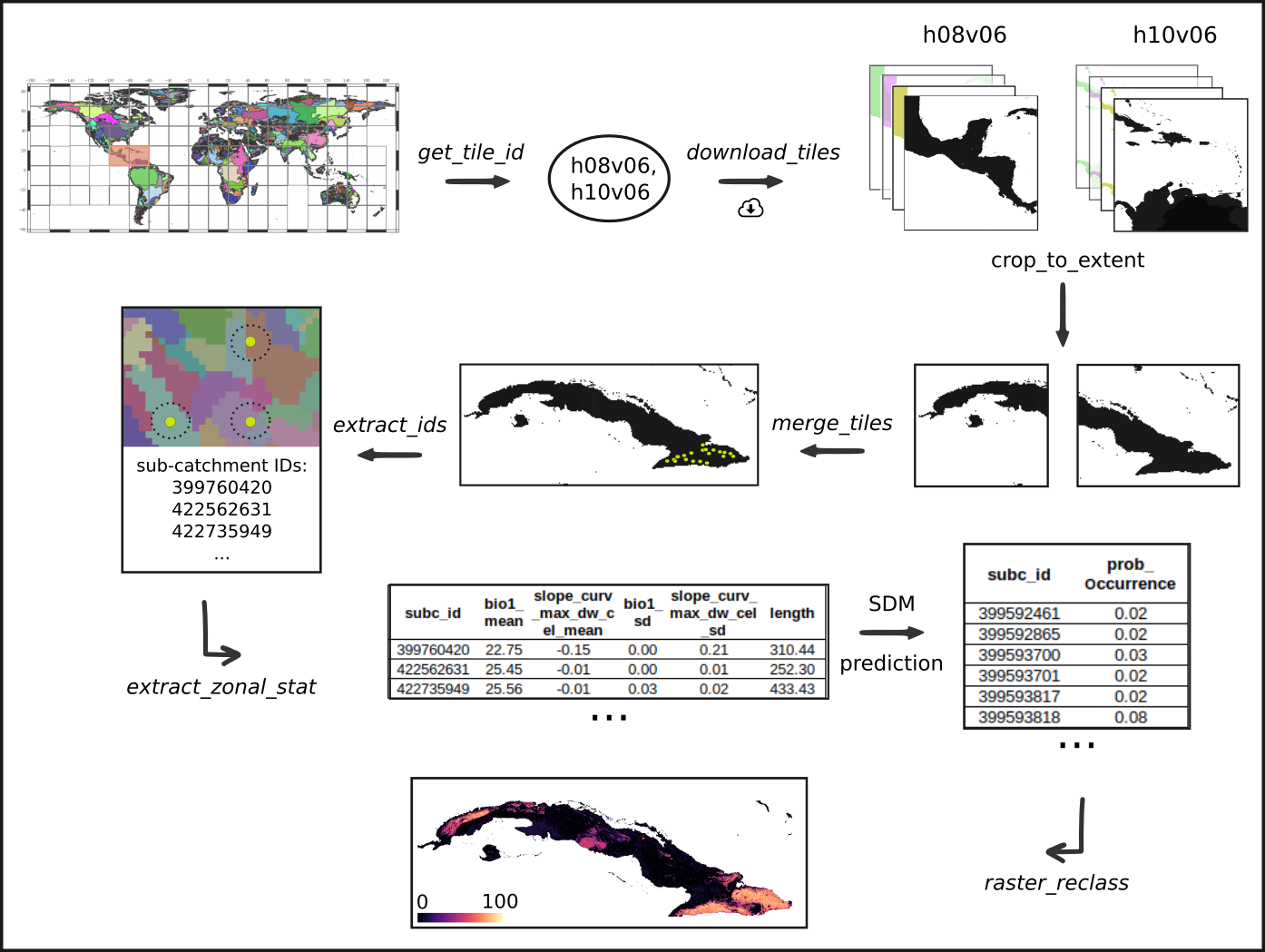
The following example showcases the functionality of the hydrographr package along a species distribution modelling (SDM) workflow. We will use an SDM to predict the suitable habitats of a dragonfly species in Cuba. We will start by defining the regular tiles of the Hydrography90m (Amatulli et al., 2022) where the occurrence points of the species are located. Afterwards we will download the Hydrography90m and CHELSA Bioclim (Karger & Zimmermann, 2019) layers of the predictor variables, crop them and merge them, if necessary. Then, we will aggregate the variable values within each sub-catchment of the study area, keeping as predictors their mean and SD per sub-catchment. Using the random forest (RF) algorithm, we will build a simple SDM and predict where the species could potentially occur. Finally, we will reclassify the layer of all the sub-catchments in the study area, creating a habitat suitability map.

Hypolestes trinitatis is a damselfly species endemic to Cuba. The species inhabits rivers and streams located in forest areas at the main mountain ranges of eastern and central Cuba. The presence of riparian forests as well as clean and well oxygenated water seems to be important ecological conditions required by H. trinitatis. Larvae can be found clinging to boulders and cobbles in the river bed at fast-flowing water stream segments and pre-reproductive adults of both sexes and sexually mature females remain most of the time in the vegetation of the riparian forest where they find shelter and prey.

Let’s get started!

Load required libraries

library(hydrographr)
library(data.table)
library(dplyr)
library(terra)
library(tools)
library(stringr)
library(ranger)
library(leaflet)
library(leafem)

Define working directory

# Define the "data_cuba" directory, where you have downloaded all the data,
# as the working directory
wdir <- "my/working/directory/data_cuba"
setwd(wdir)

# Create a new folder in the working directory to store all the data
dir.create("data")

Species data

We will start by downloading a dataset including aquatic insect occurrence records in Cuba from https://doi.org/10.18728/igb-fred-778.3 (Cambas & Salina, 2022).

download.file("https://fred.igb-berlin.de/data/file_download/1395",
              destfile = paste0(wdir, "/data/spdata_cuba.csv"), mode = "wb")

Import the dataset and select the occurrences of the species of interest, sampled after the year 1980 (to match with the climate data)

spdata <- fread(paste0(wdir, "/data/spdata_cuba.csv"), sep = "\t", fill = TRUE) %>%
          filter(species == "Hypolestes_trinitatis") %>%
          filter(year > 1980)

Subset columns

spdata <- spdata %>%
  dplyr::select(c("occurrence_ID", "species", "longitude", "latitude", "year"))

spdata

occurrence_ID	species	longitude	latitude	year
107705340	Hypolestes_trinitatis	-75.73	20.01	2006
107705519	Hypolestes_trinitatis	-75.37	20.40	2003
107705533	Hypolestes_trinitatis	-75.78	20.50	1998
107705535	Hypolestes_trinitatis	-77.03	20.20	1998
107705546	Hypolestes_trinitatis	-74.81	20.44	2008
107705657	Hypolestes_trinitatis	-75.76	20.09	2012
107705727	Hypolestes_trinitatis	-80.06	21.96	2015
107705733	Hypolestes_trinitatis	-76.04	20.03	2011
107705744	Hypolestes_trinitatis	-74.71	20.44	2004
107705863	Hypolestes_trinitatis	-75.76	20.09	2004
107706093	Hypolestes_trinitatis	-76.77	20.00	1996
107706107	Hypolestes_trinitatis	-75.44	20.58	2001
107706146	Hypolestes_trinitatis	-75.34	20.53	2001
107706216	Hypolestes_trinitatis	-75.44	20.58	2001
107706217	Hypolestes_trinitatis	-75.53	20.54	2001
107706218	Hypolestes_trinitatis	-75.53	20.54	2001
107706240	Hypolestes_trinitatis	-76.31	20.21	2003
107706332	Hypolestes_trinitatis	-75.77	20.41	2001
107706355	Hypolestes_trinitatis	-75.66	20.61	2001
107706359	Hypolestes_trinitatis	-75.66	20.46	2001
107706363	Hypolestes_trinitatis	-75.74	20.58	2000
107706366	Hypolestes_trinitatis	-75.65	20.60	2001
107706369	Hypolestes_trinitatis	-75.64	20.65	2000
107706370	Hypolestes_trinitatis	-75.69	20.60	1999
107706375	Hypolestes_trinitatis	-75.71	20.44	2000
107706378	Hypolestes_trinitatis	-75.77	20.45	1999
107706384	Hypolestes_trinitatis	-75.65	20.60	2001
107706385	Hypolestes_trinitatis	-75.65	20.60	2001
107706386	Hypolestes_trinitatis	-75.66	20.46	2000
107706387	Hypolestes_trinitatis	-75.66	20.46	2001
107706388	Hypolestes_trinitatis	-75.77	20.45	1999
107706420	Hypolestes_trinitatis	-76.11	20.07	2005
107706436	Hypolestes_trinitatis	-74.84	20.43	1998
107706561	Hypolestes_trinitatis	-75.37	20.40	2004
107706589	Hypolestes_trinitatis	-77.04	20.09	1998
107706709	Hypolestes_trinitatis	-74.99	20.48	2003
107706715	Hypolestes_trinitatis	-75.39	20.57	2004
107706720	Hypolestes_trinitatis	-76.66	20.04	2004
107706807	Hypolestes_trinitatis	-75.06	20.46	2003
107706909	Hypolestes_trinitatis	-75.70	19.96	2001
107706916	Hypolestes_trinitatis	-75.75	20.05	1996
107706937	Hypolestes_trinitatis	-74.91	20.39	2003
107706938	Hypolestes_trinitatis	-75.13	20.52	2003

Let’s visualise the species occurrences on the map

# Convert species data to a spatial vector object to plot the points
spdata_vect <- vect(spdata, geom=c("longitude", "latitude"))

Let’s define the extent (bounding box) of the study area (xmin, ymin, xmax, ymax)

bbox <- c(-84.9749110583, 19.8554808619, -74.1780248685, 23.1886107447)

m <- leaflet() %>%
  addProviderTiles('Esri.WorldShadedRelief') %>%
  setMaxBounds(bbox[1], bbox[2], bbox[3], bbox[4]) %>%
  addCircles(data = spdata_vect, color = "purple") # data = spdata

m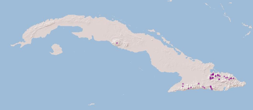

Download files

In order to download layers of the Hydrography90m, we need to know the IDs of the 20°x20° tiles in which they are located. We can obtain these IDs using the function get_tile_id(). This function downloads and uses the auxiliary raster file that contains all the regional units globally, and thus requires an active internet connection.

tile_id <- get_tile_id(data = spdata, lon = "longitude", lat = "latitude")

tile_id

## [1] "h08v06" "h10v04" "h10v06"

Currently the function returns all the tiles of the regional unit where the input points are located. However, some of them may be far from the study area and hence not always needed in further steps. Please double check which tile IDs are relevant for your purpose using the Tile map found here.

In our case, Cuba spreads across two tiles, which hold the IDs “h08v06” and “h10v06”, so we will keep only these two.

tile_id <- tile_id[c(1,3)]

Let’s define the Hydrography90m variables that we would like to download. We will use the variables slope_curv_max_dw_cel (maximum curvature between the highest upstream, focal and downstream cell) and spi (Stream Power Index) and stream length as predictors in our model.

Additionally, we will download the sub_catchment layer, which is the necessary base-layer for the workflow.

A list of all available Hydrography90m variables, as well as details and visualisations are available here.

# Variables in raster format
vars_tif <- c("sub_catchment", "slope_curv_max_dw_cel", "spi")
# Variables in vector format. This layerholds the information on stream length
vars_gpkg <- c("order_vect_point")

# Download the .tif tiles of the desired variables
download_tiles(variable = vars_tif, tile_id = tile_id, file_format = "tif",
              download_dir = "data")

# Download the .gpkg tiles of the desired variables
download_tiles(variable = vars_gpkg, tile_id = tile_id, file_format = "gpkg",
              download_dir = "data")

Then download the CHELSA present and future Bioclim variables

For a quick outlook on the bioclimatic variables you can have a look here.

# Create download directory
dir.create(paste0(wdir, "/data/chelsa_bioclim"))

# Extend timeout to 1000s to allow uninterrupted downloading
options(timeout = 1000)

# Download
# Present, 1981-2010
download.file("https://os.zhdk.cloud.switch.ch/envicloud/chelsa/chelsa_V2/GLOBAL/climatologies/1981-2010/bio/CHELSA_bio12_1981-2010_V.2.1.tif",
destfile = "data/chelsa_bioclim/bio12_1981-2010.tif", mode = "wb")
download.file("https://os.zhdk.cloud.switch.ch/envicloud/chelsa/chelsa_V2/GLOBAL/climatologies/1981-2010/bio/CHELSA_bio15_1981-2010_V.2.1.tif",
destfile = "data/chelsa_bioclim/bio15_1981-2010.tif", mode = "wb")
download.file("https://os.zhdk.cloud.switch.ch/envicloud/chelsa/chelsa_V2/GLOBAL/climatologies/1981-2010/bio/CHELSA_bio1_1981-2010_V.2.1.tif",
destfile = "data/chelsa_bioclim/bio1_1981-2010.tif", mode = "wb")
# Future, 2041-2070
download.file("https://os.zhdk.cloud.switch.ch/envicloud/chelsa/chelsa_V2/GLOBAL/climatologies/2041-2070/IPSL-CM6A-LR/ssp370/bio/CHELSA_bio12_2041-2070_ipsl-cm6a-lr_ssp370_V.2.1.tif",
destfile = "data/chelsa_bioclim/bio12_IPSL-CM6A-LR_ssp370_2041-2070.tif", mode = "wb")
download.file("https://os.zhdk.cloud.switch.ch/envicloud/chelsa/chelsa_V2/GLOBAL/climatologies/2041-2070/IPSL-CM6A-LR/ssp370/bio/CHELSA_bio15_2041-2070_ipsl-cm6a-lr_ssp370_V.2.1.tif",
destfile = "data/chelsa_bioclim/bio15_IPSL-CM6A-LR_ssp370_2041-2070.tif", mode = "wb")
download.file("https://os.zhdk.cloud.switch.ch/envicloud/chelsa/chelsa_V2/GLOBAL/climatologies/2041-2070/IPSL-CM6A-LR/ssp370/bio/CHELSA_bio1_2041-2070_ipsl-cm6a-lr_ssp370_V.2.1.tif",
destfile = "data/chelsa_bioclim/bio1_IPSL-CM6A-LR_ssp370_2041-2070.tif", mode = "wb")

Cropping

After having downloaded all the layers, we need to crop them to the extent of our study area. This is straightforward in the case of the global CHELSA layers:

We define the directory containing the layers to be cropped

dirs_chelsa <- paste0(wdir, "/data/chelsa_bioclim")

… and the final output directory

# Define output directory for merged files
layer_dir <- paste0(wdir, "/data/final_layers")
# Create the directory
dir.create(layer_dir)

We then crop the files using the function crop_to_extent() in a loop

files_chelsa <- list.files(dirs_chelsa, pattern = ".tif", full.names = TRUE)

for(ifile in files_chelsa) {
    crop_to_extent(
      raster_layer = ifile,
      bounding_box = bbox,
      out_dir = layer_dir,
      file_name = basename(ifile),
      read = FALSE,
      quiet = TRUE)
}

However, the hydrographic variable slope_curv_max_dw_cel (the maximum curvature between the highest upstream, the focal, and the downstream cell) is split across two tiles. We highly recommend to first crop the tiles to the extent of the study area to limit their size, and afterwards merge them into one file.

Again, we will first define the input directories, but this time we will store the cropped files in the same directory as the input files, as there is an extra step before reaching to the final output.

dirs_h90m <- list.dirs(paste0(wdir, "/data"),
                       recursive = TRUE, full.names = TRUE)

dirs_h90m <- dirs_h90m[grep("tiles20d", dirs_h90m)]

for(idir in dirs_h90m) {
  # only choose rasters
  tiles <- list.files(idir, pattern = ".tif$", full.names = TRUE)
  for(itile in tiles) {
      crop_to_extent(
        raster_layer = itile,
        bounding_box = bbox,
        out_dir = idir,
        file_name = paste0(str_remove(basename(itile), ".tif"), "_crop.tif"),
        read = FALSE,
        quiet = TRUE)
  }
}

Merging

The cropped tiles of the variable now need to be merged together.

# This can be done sequentially:
idir <- dirs_h90m[1]
merge_tiles(tile_dir = idir,
            tile_names = list.files(idir, full.names = FALSE,
                                    pattern = "_crop.tif"),
            out_dir = layer_dir,
            file_name = "spi.tif",
            read = FALSE)

idir <- dirs_h90m[3]
merge_tiles(tile_dir = idir,
            tile_names = list.files(idir, full.names = FALSE,
                                    pattern = "_crop.tif"),
            out_dir = layer_dir,
            file_name = "slope_curv_max_dw_cel.tif",
            read = FALSE)

idir <- dirs_h90m[4]
merge_tiles(tile_dir = idir,
            tile_names = list.files(idir, full.names = FALSE,
                                    pattern = "_crop.tif"),
            out_dir = layer_dir,
            file_name = "sub_catchment.tif",
            read = FALSE)



# ...or in a loop
for(idir in dirs_h90m[c(1,3,4)]) {
  # Get input file extension
  file_extension <- file_ext(list.files(idir, full.names = FALSE)[1])

  # Assign file extension to output files
  ivar_name <- paste0(
    str_remove(basename(idir), "_tiles20d"), ".", file_extension
  )

  # Run the function
  merge_tiles(tile_dir = idir,
              tile_names = list.files(idir, full.names = FALSE,
                                      pattern = "_crop.tif"),
              out_dir = layer_dir,
              file_name = ivar_name,
              read = FALSE, 
              bigtiff = TRUE)
}

Extraction of sub-catchment IDs

Extract the IDs of the sub-catchments where the points are located. This step is crucial, as many of the functions that we will later use require a vector of sub-catchment IDs as input. Note that the function extract_ids() can be used to extract the values at specific points of any raster file provided to the argument subc_layer. It can be safely used to query very large raster files, as these are not loaded into R.

spdata_ids <- extract_ids(data = spdata, lon = "longitude", lat = "latitude",
                          id = "occurrence_ID", quiet = FALSE,
                          subc_layer = paste0(layer_dir, "/sub_catchment.tif"))

The species data have now their corresponding sub-catchment ids
longitude	latitude	occurrence_ID	subcatchment_id
-75.73	20.01	107705340	422886180
-75.37	20.40	107705519	422816272
-75.78	20.50	107705533	422801107
-77.03	20.20	107705535	422851157
-74.81	20.44	107705546	422809465
-75.76	20.09	107705657	422872031

Aggregation of environmental layers

We will calculate the zonal statistics of the Hydrography90m and the CHELSA Bioclim variables for all the sub-catchments of the study area. Caution, don’t increase the number of cores to more than 3 as this can cause memory problems. However, this highly depends to the number of sub-catchments as well. We recommend to test the function with different parameters to find out what works best for your case.

# Define input var_layers for the extract_zonal_stat() function
var_layers <- list.files(layer_dir)[-9]
# var_layers <- list.files(layer_dir)[c(3,5,7)]
var_layers

## [1] "bio1_1981-2010.tif"                     
## [2] "bio1_IPSL-CM6A-LR_ssp370_2041-2070.tif"
## [3] "bio12_1981-2010.tif"                    
## [4] "bio12_IPSL-CM6A-LR_ssp370_2041-2070.tif"
## [5] "bio15_1981-2010.tif"                    
## [6] "bio15_IPSL-CM6A-LR_ssp370_2041-2070.tif"
## [7] "slope_curv_max_dw_cel.tif"              
## [8] "spi.tif"

A good practice before aggregating the variables is to check their NoData values:

report_no_data(data_dir = layer_dir, var_layer = var_layers)

##                                    Raster   NoData
## 1                     bio15_1981-2010.tif        0
## 2                      bio1_1981-2010.tif        0
## 3  bio1_IPSL-CM6A-LR_ssp370_2041-2070.tif        0
## 4                     bio12_1981-2010.tif        0
## 5 bio12_IPSL-CM6A-LR_ssp370_2041-2070.tif        0
## 6 bio15_IPSL-CM6A-LR_ssp370_2041-2070.tif        0
## 7               slope_curv_max_dw_cel.tif -9999999
## 8                                 spi.tif -9999999

# Run the function that returns the zonal statistics
stats_table_zon <- extract_zonal_stat(
                    data_dir = layer_dir,
                    subc_layer = paste0(layer_dir, "/sub_catchment.tif"),
                    subc_id = "all",
                    var_layer = var_layers,
                    out_dir = paste0(wdir, "/data"),
                    file_name = "zonal_stats.csv",
                    n_cores = 2)

The function also reports the NoData values that are used in the calculation of the zonal statistics of each variable.

# Read the previously created file
stats_table_zon <- fread(paste0(wdir, "/data/zonal_stats.csv"))

Let’s inspect the resulting table

subc_id	bio1_1981.2010_data_cells	bio1_1981.2010_min	bio1_1981.2010_max	bio1_1981.2010_mean	bio1_1981.2010_mean_abs	bio1_1981.2010_sum	bio1_1981.2010_sum_abs	bio1_IPSL.CM6A.LR_ssp370_2041.2070_data_cells	bio1_IPSL.CM6A.LR_ssp370_2041.2070_min	bio1_IPSL.CM6A.LR_ssp370_2041.2070_max	bio1_IPSL.CM6A.LR_ssp370_2041.2070_mean	bio1_IPSL.CM6A.LR_ssp370_2041.2070_mean_abs	bio1_IPSL.CM6A.LR_ssp370_2041.2070_sum	bio1_IPSL.CM6A.LR_ssp370_2041.2070_sum_abs	bio12_1981.2010_data_cells	bio12_1981.2010_min	bio12_1981.2010_max	bio12_1981.2010_range	bio12_1981.2010_mean	bio12_1981.2010_mean_abs	bio12_1981.2010_sd	bio12_1981.2010_var	bio12_1981.2010_cv	bio12_1981.2010_sum	bio12_1981.2010_sum_abs	bio12_IPSL.CM6A.LR_ssp370_2041.2070_data_cells	bio12_IPSL.CM6A.LR_ssp370_2041.2070_min	bio12_IPSL.CM6A.LR_ssp370_2041.2070_max	bio12_IPSL.CM6A.LR_ssp370_2041.2070_range	bio12_IPSL.CM6A.LR_ssp370_2041.2070_mean	bio12_IPSL.CM6A.LR_ssp370_2041.2070_mean_abs	bio12_IPSL.CM6A.LR_ssp370_2041.2070_sd	bio12_IPSL.CM6A.LR_ssp370_2041.2070_var	bio12_IPSL.CM6A.LR_ssp370_2041.2070_cv	bio12_IPSL.CM6A.LR_ssp370_2041.2070_sum	bio12_IPSL.CM6A.LR_ssp370_2041.2070_sum_abs	bio15_1981.2010_data_cells	bio15_1981.2010_min	bio15_1981.2010_max	bio15_1981.2010_range	bio15_1981.2010_mean	bio15_1981.2010_mean_abs	bio15_1981.2010_sd	bio15_1981.2010_var	bio15_1981.2010_cv	bio15_1981.2010_sum	bio15_1981.2010_sum_abs	bio15_IPSL.CM6A.LR_ssp370_2041.2070_data_cells	bio15_IPSL.CM6A.LR_ssp370_2041.2070_min	bio15_IPSL.CM6A.LR_ssp370_2041.2070_max	bio15_IPSL.CM6A.LR_ssp370_2041.2070_range	bio15_IPSL.CM6A.LR_ssp370_2041.2070_mean	bio15_IPSL.CM6A.LR_ssp370_2041.2070_mean_abs	bio15_IPSL.CM6A.LR_ssp370_2041.2070_sd	bio15_IPSL.CM6A.LR_ssp370_2041.2070_var	bio15_IPSL.CM6A.LR_ssp370_2041.2070_cv	bio15_IPSL.CM6A.LR_ssp370_2041.2070_sum	bio15_IPSL.CM6A.LR_ssp370_2041.2070_sum_abs	slope_curv_max_dw_cel_data_cells	slope_curv_max_dw_cel_nodata_cells	slope_curv_max_dw_cel_min	slope_curv_max_dw_cel_max	slope_curv_max_dw_cel_range	slope_curv_max_dw_cel_mean	slope_curv_max_dw_cel_mean_abs	slope_curv_max_dw_cel_sd	slope_curv_max_dw_cel_var	slope_curv_max_dw_cel_cv	slope_curv_max_dw_cel_sum	slope_curv_max_dw_cel_sum_abs	spi_data_cells	spi_nodata_cells	spi_min	spi_max	spi_range	spi_mean	spi_mean_abs	spi_sd	spi_var	spi_cv	spi_sum	spi_sum_abs
399592461	355	2986	2986	2986	2986	1060030	1060030	355	3005	3005	3005	3005	1066775	1066775	355	11031	11084	53	11050.04	11050.04	17.799709	316.82964	0.1610828	3922763	3922763	355	10532	10575	43	10546.23	10546.23	13.81320	190.80449	0.1309776	3743913	3743913	355	414	416	2	414.7380	414.7380	0.9650755	0.9313708	0.2326952	147232	147232	355	373	375	2	374.0225	374.0225	0.6230767	0.3882246	0.1665880	132778	132778	354	1	-54884	30865	85749	-2472.034	5752.051	12038.554	144926775	-486.9898	-875100	2036226	354	1	0	44	44	6.655367	6.655367	9.411190	88.570494	141.40752	2356	2356
399592865	82	2986	2986	2986	2986	244852	244852	82	3005	3005	3005	3005	246410	246410	82	11042	11084	42	11049.17	11049.17	9.880758	97.62939	0.0894253	906032	906032	82	10540	10575	35	10545.72	10545.72	8.19023	67.07986	0.0776640	864749	864749	82	414	416	2	414.1220	414.1220	0.4785711	0.2290303	0.1155629	33958	33958	82	373	374	1	373.0610	373.0610	0.2392856	0.0572576	0.0641411	30591	30591	81	1	-40084	18444	58528	-3907.630	7527.259	12947.641	167641415	-331.3426	-316518	609708	81	1	0	70	70	8.925926	8.925926	13.105251	171.747600	146.82231	723	723
399593700	148	2986	2986	2986	2986	441928	441928	148	3005	3005	3005	3005	444740	444740	148	11008	11054	46	11019.70	11019.70	14.048015	197.34674	0.1274810	1630915	1630915	148	10510	10548	38	10520.42	10520.42	11.55306	133.47316	0.1098156	1557022	1557022	148	414	416	2	414.5811	414.5811	0.8055006	0.6488313	0.1942927	61358	61358	148	375	376	1	375.1757	375.1757	0.3805440	0.1448137	0.1014309	55526	55526	148	0	-28093	14059	42152	-1160.236	3082.331	7115.013	50623405	-613.2381	-171715	456185	148	0	0	12	12	2.439189	2.439189	2.916000	8.503059	119.54794	361	361
399593701	7	2986	2986	2986	2986	20902	20902	7	3005	3005	3005	3005	21035	21035	7	10987	10987	0	10987.00	10987.00	0.000000	0.00000	0.0000000	76909	76909	7	10490	10490	0	10490.00	10490.00	0.00000	0.00000	0.0000000	73430	73430	7	415	415	0	415.0000	415.0000	0.0000000	0.0000000	0.0000000	2905	2905	7	376	376	0	376.0000	376.0000	0.0000000	0.0000000	0.0000000	2632	2632	7	0	-8035	5997	14032	-2046.286	3874.571	4235.546	17939850	-206.9870	-14324	27122	7	0	0	10	10	2.142857	2.142857	3.481731	12.122449	162.48077	15	15
399593817	162	2986	2986	2986	2986	483732	483732	162	3005	3005	3005	3005	486810	486810	162	10993	11042	49	11009.02	11009.02	14.746614	217.46262	0.1339503	1783461	1783461	162	10496	10537	41	10509.90	10509.90	12.24907	150.03963	0.1165479	1702604	1702604	162	414	416	2	414.7654	414.7654	0.7161558	0.5128791	0.1726653	67192	67192	162	375	376	1	375.2160	375.2160	0.4115484	0.1693720	0.1096830	60785	60785	162	0	-38488	19276	57764	-2234.920	5134.846	9093.644	82694353	-406.8890	-362057	831845	162	0	0	19	19	2.660494	2.660494	3.961487	15.693378	148.90043	431	431
399593818	5	2986	2986	2986	2986	14930	14930	5	3005	3005	3005	3005	15025	15025	5	10975	10987	12	10977.40	10977.40	4.800000	23.04000	0.0437262	54887	54887	5	10479	10490	11	10481.20	10481.20	4.40000	19.36000	0.0419799	52406	52406	5	415	415	0	415.0000	415.0000	0.0000000	0.0000000	0.0000000	2075	2075	5	376	377	1	376.8000	376.8000	0.4000000	0.1600000	0.1061571	1884	1884	5	0	0	10582	10582	2116.400	2116.400	4232.800	17916596	200.0000	10582	10582	5	0	1	2	1	1.200000	1.200000	0.400000	0.160000	33.33333	6	6

colnames(stats_table_zon)

##  [1] "subc_id"                                         
##  [2] "bio1_1981.2010_data_cells"                       
##  [3] "bio1_1981.2010_nodata_cells"                     
##  [4] "bio1_1981.2010_min"                              
##  [5] "bio1_1981.2010_max"                              
##  [6] "bio1_1981.2010_range"                            
##  [7] "bio1_1981.2010_mean"                             
##  [8] "bio1_1981.2010_mean_abs"                         
##  [9] "bio1_1981.2010_sd"                               
## [10] "bio1_1981.2010_var"                              
## [11] "bio1_1981.2010_cv"                               
## [12] "bio1_1981.2010_sum"                              
## [13] "bio1_1981.2010_sum_abs"                          
## [14] "bio1_IPSL.CM6A.LR_ssp370_2041.2070_data_cells"   
## [15] "bio1_IPSL.CM6A.LR_ssp370_2041.2070_nodata_cells" 
## [16] "bio1_IPSL.CM6A.LR_ssp370_2041.2070_min"          
## [17] "bio1_IPSL.CM6A.LR_ssp370_2041.2070_max"          
## [18] "bio1_IPSL.CM6A.LR_ssp370_2041.2070_range"        
## [19] "bio1_IPSL.CM6A.LR_ssp370_2041.2070_mean"         
## [20] "bio1_IPSL.CM6A.LR_ssp370_2041.2070_mean_abs"     
## [21] "bio1_IPSL.CM6A.LR_ssp370_2041.2070_sd"           
## [22] "bio1_IPSL.CM6A.LR_ssp370_2041.2070_var"          
## [23] "bio1_IPSL.CM6A.LR_ssp370_2041.2070_cv"           
## [24] "bio1_IPSL.CM6A.LR_ssp370_2041.2070_sum"          
## [25] "bio1_IPSL.CM6A.LR_ssp370_2041.2070_sum_abs"      
## [26] "bio12_1981.2010_data_cells"                      
## [27] "bio12_1981.2010_nodata_cells"                    
## [28] "bio12_1981.2010_min"                             
## [29] "bio12_1981.2010_max"                             
## [30] "bio12_1981.2010_range"                           
## [31] "bio12_1981.2010_mean"                            
## [32] "bio12_1981.2010_mean_abs"                        
## [33] "bio12_1981.2010_sd"                              
## [34] "bio12_1981.2010_var"                             
## [35] "bio12_1981.2010_cv"                              
## [36] "bio12_1981.2010_sum"                             
## [37] "bio12_1981.2010_sum_abs"                         
## [38] "bio12_IPSL.CM6A.LR_ssp370_2041.2070_data_cells"  
## [39] "bio12_IPSL.CM6A.LR_ssp370_2041.2070_nodata_cells"
## [40] "bio12_IPSL.CM6A.LR_ssp370_2041.2070_min"         
## [41] "bio12_IPSL.CM6A.LR_ssp370_2041.2070_max"         
## [42] "bio12_IPSL.CM6A.LR_ssp370_2041.2070_range"       
## [43] "bio12_IPSL.CM6A.LR_ssp370_2041.2070_mean"        
## [44] "bio12_IPSL.CM6A.LR_ssp370_2041.2070_mean_abs"    
## [45] "bio12_IPSL.CM6A.LR_ssp370_2041.2070_sd"          
## [46] "bio12_IPSL.CM6A.LR_ssp370_2041.2070_var"         
## [47] "bio12_IPSL.CM6A.LR_ssp370_2041.2070_cv"          
## [48] "bio12_IPSL.CM6A.LR_ssp370_2041.2070_sum"         
## [49] "bio12_IPSL.CM6A.LR_ssp370_2041.2070_sum_abs"     
## [50] "bio15_1981.2010_data_cells"                      
## [51] "bio15_1981.2010_nodata_cells"                    
## [52] "bio15_1981.2010_min"                             
## [53] "bio15_1981.2010_max"                             
## [54] "bio15_1981.2010_range"                           
## [55] "bio15_1981.2010_mean"                            
## [56] "bio15_1981.2010_mean_abs"                        
## [57] "bio15_1981.2010_sd"                              
## [58] "bio15_1981.2010_var"                             
## [59] "bio15_1981.2010_cv"                              
## [60] "bio15_1981.2010_sum"                             
## [61] "bio15_1981.2010_sum_abs"                         
## [62] "bio15_IPSL.CM6A.LR_ssp370_2041.2070_data_cells"  
## [63] "bio15_IPSL.CM6A.LR_ssp370_2041.2070_nodata_cells"
## [64] "bio15_IPSL.CM6A.LR_ssp370_2041.2070_min"         
## [65] "bio15_IPSL.CM6A.LR_ssp370_2041.2070_max"         
## [66] "bio15_IPSL.CM6A.LR_ssp370_2041.2070_range"       
## [67] "bio15_IPSL.CM6A.LR_ssp370_2041.2070_mean"        
## [68] "bio15_IPSL.CM6A.LR_ssp370_2041.2070_mean_abs"    
## [69] "bio15_IPSL.CM6A.LR_ssp370_2041.2070_sd"          
## [70] "bio15_IPSL.CM6A.LR_ssp370_2041.2070_var"         
## [71] "bio15_IPSL.CM6A.LR_ssp370_2041.2070_cv"          
## [72] "bio15_IPSL.CM6A.LR_ssp370_2041.2070_sum"         
## [73] "bio15_IPSL.CM6A.LR_ssp370_2041.2070_sum_abs"     
## [74] "slope_curv_max_dw_cel_data_cells"                
## [75] "slope_curv_max_dw_cel_nodata_cells"              
## [76] "slope_curv_max_dw_cel_min"                       
## [77] "slope_curv_max_dw_cel_max"                       
## [78] "slope_curv_max_dw_cel_range"                     
## [79] "slope_curv_max_dw_cel_mean"                      
## [80] "slope_curv_max_dw_cel_mean_abs"                  
## [81] "slope_curv_max_dw_cel_sd"                        
## [82] "slope_curv_max_dw_cel_var"                       
## [83] "slope_curv_max_dw_cel_cv"                        
## [84] "slope_curv_max_dw_cel_sum"                       
## [85] "slope_curv_max_dw_cel_sum_abs"                   
## [86] "spi_data_cells"                                  
## [87] "spi_nodata_cells"                                
## [88] "spi_min"                                         
## [89] "spi_max"                                         
## [90] "spi_range"                                       
## [91] "spi_mean"                                        
## [92] "spi_mean_abs"                                    
## [93] "spi_sd"                                          
## [94] "spi_var"                                         
## [95] "spi_cv"                                          
## [96] "spi_sum"                                         
## [97] "spi_sum_abs"

We will keep only the mean and sd of each variable of the stats_table, to use them as predictors in the species distribution model

stats_table_zon <- stats_table_zon %>%
  dplyr::select(contains("subc") |  ends_with("_mean") | ends_with("_sd")) %>%
  rename('subcatchment_id' = 'subc_id')

Reading vector files

Read in the .gpkg databases of the two tiles, filtering only the sub-catchments of the study area. Their IDs can be retrieved from the stats_table

stats_gpkg_h08v06 <- read_geopackage(
  "data/r.stream.order/order_vect_tiles20d/order_vect_point_h08v06.gpkg",
  subc_id = stats_table_zon$subcatchment_id) %>%
  rename('subcatchment_id' = 'stream')

stats_gpkg_h10v06 <- read_geopackage(
  "data/r.stream.order/order_vect_tiles20d/order_vect_point_h10v06.gpkg",
  subc_id = stats_table_zon$subcatchment_id) %>%
  rename('subcatchment_id' = 'stream')

Then we join the two .gpkg databases and select the columns “subcatchment_id” and “length”. We will use the length of the stream as an indicator of the sub-catchment size

stats_gpkg <- rbind(stats_gpkg_h08v06, stats_gpkg_h10v06) %>%
  dplyr::select(c("subcatchment_id", "length"))

# Clear up memory
rm(stats_gpkg_h08v06, stats_gpkg_h10v06); gc()

##            used  (Mb) gc trigger  (Mb)  max used  (Mb)
## Ncells  4627996 247.2    8678052 463.5   7056390 376.9
## Vcells 27081171 206.7   83906542 640.2 104364691 796.3

Prepare data for modelling

Join the stats_table with the .gpkg database

stats_table <- left_join(stats_table_zon, stats_gpkg, by = "subcatchment_id")

The values in the original raster files were scaled, so we need to re-scale them before the modelling

We define the following functions:

slope_scale <- function(x, na.rm = F) (x * 0.000001)
clim_scale <- function(x, na.rm = F) (x * 0.1)
offset <- function(x, na.rm = F) (x - 273.15)

… and apply them to rescale the values

stats_table <- stats_table  %>%
  mutate(across(contains("slope_curv_max_dw_cel"), slope_scale)) %>%
  mutate(across(starts_with("bio"), clim_scale))  %>%
  mutate(across(matches("bio1_.*_mean"), offset))

head(stats_table)

subcatchment_id	bio1_1981.2010_mean	bio1_IPSL.CM6A.LR_ssp370_2041.2070_mean	bio12_1981.2010_mean	bio12_IPSL.CM6A.LR_ssp370_2041.2070_mean	bio15_1981.2010_mean	bio15_IPSL.CM6A.LR_ssp370_2041.2070_mean	slope_curv_max_dw_cel_mean	spi_mean	bio12_1981.2010_sd	bio12_IPSL.CM6A.LR_ssp370_2041.2070_sd	bio15_1981.2010_sd	bio15_IPSL.CM6A.LR_ssp370_2041.2070_sd	slope_curv_max_dw_cel_sd	spi_sd	length
399592461	25.45	27.35	1105.004	1054.623	41.47380	37.40225	-0.0024720	6.655367	1.7799709	1.381320	0.0965076	0.0623077	0.0120386	9.411190	3827.3302
399592865	25.45	27.35	1104.917	1054.572	41.41220	37.30610	-0.0039076	8.925926	0.9880758	0.819023	0.0478571	0.0239286	0.0129476	13.105251	2911.9507
399593700	25.45	27.35	1101.970	1052.042	41.45811	37.51757	-0.0011602	2.439189	1.4048016	1.155306	0.0805501	0.0380544	0.0071150	2.916000	1903.8027
399593701	25.45	27.35	1098.700	1049.000	41.50000	37.60000	-0.0020463	2.142857	0.0000000	0.000000	0.0000000	0.0000000	0.0042355	3.481731	1057.3782
399593817	25.45	27.35	1100.902	1050.990	41.47654	37.52160	-0.0022349	2.660494	1.4746614	1.224907	0.0716156	0.0411548	0.0090936	3.961487	2343.3823
399593818	25.45	27.35	1097.740	1048.120	41.50000	37.68000	0.0021164	1.200000	0.4800000	0.440000	0.0000000	0.0400000	0.0042328	0.400000	812.9898

head(stats_table[is.na(stats_table$slope_curv_max_dw_cel_mean),])

subcatchment_id	bio1_1981.2010_mean	bio1_IPSL.CM6A.LR_ssp370_2041.2070_mean	bio12_1981.2010_mean	bio12_IPSL.CM6A.LR_ssp370_2041.2070_mean	bio15_1981.2010_mean	bio15_IPSL.CM6A.LR_ssp370_2041.2070_mean	slope_curv_max_dw_cel_mean	spi_mean	slope_curv_max_dw_cel_sd	spi_sd
399596764	25.45	27.35	1110.4	1054.3	41.8	36.6	NA	NA	NA	NA
399597046	25.55	27.55	1362.3	1261.1	49.3	42.9	NA	NA	NA	NA
399604194	25.35	27.35	1117.2	1059.8	42.9	38.9	NA	NA	NA	NA
399607973	25.35	27.25	1130.5	1074.5	43.2	38.6	NA	NA	NA	NA
399611470	25.35	27.25	1149.3	1086.0	44.5	39.0	NA	NA	NA	NA
399614825	25.45	27.45	1305.2	1207.6	50.2	43.9	NA	NA	NA	NA

head(stats_table[is.na(stats_table$spi_mean),])

subcatchment_id	bio1_1981.2010_mean	bio1_IPSL.CM6A.LR_ssp370_2041.2070_mean	bio12_1981.2010_mean	bio12_IPSL.CM6A.LR_ssp370_2041.2070_mean	bio15_1981.2010_mean	bio15_IPSL.CM6A.LR_ssp370_2041.2070_mean	slope_curv_max_dw_cel_mean	spi_mean	slope_curv_max_dw_cel_sd	spi_sd
399596764	25.45	27.35	1110.4	1054.3	41.8	36.6	NA	NA	NA	NA
399597046	25.55	27.55	1362.3	1261.1	49.3	42.9	NA	NA	NA	NA
399604194	25.35	27.35	1117.2	1059.8	42.9	38.9	NA	NA	NA	NA
399607973	25.35	27.25	1130.5	1074.5	43.2	38.6	NA	NA	NA	NA
399611470	25.35	27.25	1149.3	1086.0	44.5	39.0	NA	NA	NA	NA
399614825	25.45	27.45	1305.2	1207.6	50.2	43.9	NA	NA	NA	NA

If we check the IDs of the sub-catchments that have null values for both variables, we observe that they are identical:

stats_table[is.na(stats_table$spi_mean),]$subcatchment_id == stats_table[is.na(stats_table$slope_curv_max_dw_cel_mean),]$subcatchment_id

##  [1] TRUE TRUE TRUE TRUE TRUE TRUE TRUE TRUE TRUE TRUE TRUE TRUE TRUE TRUE TRUE
## [16] TRUE TRUE TRUE TRUE TRUE TRUE TRUE TRUE TRUE TRUE TRUE TRUE TRUE TRUE TRUE
## [31] TRUE TRUE TRUE TRUE TRUE TRUE TRUE TRUE TRUE TRUE TRUE

This happens because the variables are not defined for a few single-pixel sub-catchments, which are outlets. We will remove these sub-catchments, as the model will not be able to handle the no data values.

stats_table <- stats_table[!is.na(stats_table$slope_curv_max_dw_cel_mean),]

We split the dataset into two datasets, according to present and future Bioclim variables. The first will be used in the training of the model and the second in the prediction of future suitable habitats

stats_table_present <- stats_table %>%
  dplyr::select(!contains("IPSL")) %>%
  rename(bio1_mean = bio1_1981.2010_mean,
         bio1_sd = bio1_1981.2010_sd,
         bio12_mean = bio12_1981.2010_mean,
         bio12_sd = bio12_1981.2010_sd,
         bio15_mean = bio15_1981.2010_mean,
         bio15_sd = bio15_1981.2010_sd)

stats_table_future <- stats_table %>%
  dplyr::select(!contains("1981")) %>%
  rename(bio1_mean = bio1_IPSL.CM6A.LR_ssp370_2041.2070_mean,
         bio1_sd = bio1_IPSL.CM6A.LR_ssp370_2041.2070_sd,
         bio12_mean = bio12_IPSL.CM6A.LR_ssp370_2041.2070_mean,
         bio12_sd = bio12_IPSL.CM6A.LR_ssp370_2041.2070_sd,
         bio15_mean = bio15_IPSL.CM6A.LR_ssp370_2041.2070_mean,
         bio15_sd = bio15_IPSL.CM6A.LR_ssp370_2041.2070_sd)

# Clear up memory
# rm(stats_table) ; gc()

The classification model needs at least two classes, in this case presences and absences. We will sample 10,000 random sub-catchments that will be used as pseudoabsences in the model. The filtering that takes place before the sampling assures that we will avoid sampling sub-catchments with known presences of the species

pseudoabs <- stats_table_present %>%
  filter(!subcatchment_id %in% spdata_ids$subcatchment_id) %>%
  sample_n(10000)

head(pseudoabs)

subcatchment_id	bio1_mean	bio12_mean	bio15_mean	slope_curv_max_dw_cel_mean	spi_mean	bio1_sd	bio12_sd	bio15_sd	slope_curv_max_dw_cel_sd	spi_sd	length
422793305	26.55000	1120.400	55.80000	-0.0008033	39.333333	0.000000	0.0000000	0.0000000	0.0011366	54.920144	126.7398
422488755	25.45000	1350.133	49.20000	-0.0038440	24.666667	0.000000	0.4988877	0.0000000	0.0109126	35.039660	276.8501
422753760	26.05000	1151.571	53.88571	-0.0131156	16.285714	0.000000	2.1345553	0.0349927	0.0197631	26.751311	253.2769
399918893	25.25000	1253.100	58.10000	-0.0015966	6.076923	0.000000	0.0000000	0.0000000	0.0029588	12.733732	383.5098
422721349	26.15000	1227.500	61.20000	-0.0096218	52.250000	0.000000	0.0000000	0.0000000	0.0151893	90.499655	126.5705
422551000	23.77075	1725.443	64.49623	-0.0264115	1.490566	0.048984	1.4541430	0.0581548	0.0559768	1.632484	814.5358

We join the species occurrences with the present environmental variables table

presence <- left_join(spdata_ids, stats_table_present, by = "subcatchment_id")

We then join the predictors of the presences and those of the pseudoabsences, to obtain the modelling data table

data_model <- data.table::rbindlist(list(presence, pseudoabs), fill = TRUE)

Define a binary column of presence-absence (0-1) and set it to factor

data_model$occurrence <- ifelse(!is.na(data_model$occurrence_ID), 1, 0)
data_model$occurrence <- as.factor(data_model$occurrence)

head(data_model)

longitude	latitude	occurrence_ID	subcatchment_id	bio1_mean	bio12_mean	bio15_mean	slope_curv_max_dw_cel_mean	spi_mean	bio1_sd	bio12_sd	bio15_sd	slope_curv_max_dw_cel_sd	spi_sd	length	occurrence
-75.73	20.01	107705340	422886180	25.73519	1250.785	52.50000	-0.0324294	59.8148148	0.0755410	4.513577	0.0000000	0.0783162	123.190018	388.5433	1
-75.37	20.40	107705519	422816272	24.53667	1866.747	47.82667	-0.0349241	7.2666667	0.0339935	0.883830	0.0679869	0.0576330	6.677990	434.9116	1
-75.78	20.50	107705533	422801107	22.37000	1819.280	52.28000	-0.0280889	1.8666667	0.0400000	2.560000	0.0400000	0.0361340	1.746107	300.6135	1
-77.03	20.20	107705535	422851157	26.35000	1401.500	58.50000	-0.0020064	0.3571429	0.0000000	0.000000	0.0000000	0.0026065	0.610286	311.3841	1
-74.81	20.44	107705546	422809465	24.39706	2527.112	27.59706	-0.0927082	132.1470588	0.0882353	25.733450	0.1524029	0.1779599	307.500371	514.4451	1
-75.76	20.09	107705657	422872031	24.95000	1441.100	53.60000	-0.1552392	53.7500000	0.0000000	0.000000	0.0000000	0.1703503	88.485521	126.9131	1

In this step, there are two alternatives: Either we split the data into train and test sets:

set.seed(17)

#obtain stratified training sample
train_idx <- sample(nrow(data_model), 2/3 * nrow(data_model))
data_train <- data_model[train_idx, ]
data_test <- data_model[-train_idx, ]

…or we use the whole dataset as the training set, since RF performs intrinsic evaluation in every tree

data_train <- data_model

A simple SDM using Random Forest

We will use the ranger random forest (RF) algorithm (Wright & Ziegler, 2017) to build a species distribution model. Random forest can handle huge quantities of data and is therefore scalable to larger datasets. As our dataset is highly imbalanced towards the pseudo-absence data, we will apply the down-sampling method for presence-only data in the modelling process (Valavi et al., 2021). Down-sampling works by balancing the training data, which contain significantly more absence that presence points. Following this approach, the classification-RF model will use the same number of pseudo-absences as presence points in each classification tree, by sampling with replacement (bootstrapping) from the full pseudo-absence set (Valavi et al., 2021).

Let’s define the sample size of each classification tree as a proportion of the whole training set, based on the number of presences.

# number of presence records:
pres_num <- as.numeric(table(data_train$occurrence)["1"])
sample_size <- c("0" = pres_num / nrow(data_train),
                 "1" = pres_num / nrow(data_train))
sample_size

##           0           1 
## 0.004281589 0.004281589

Run and inspect the model.

model <- ranger(data_train$occurrence ~ .,
                 data = data_train[, 6:14],
                 num.trees = 1000,
                 mtry= 6,
                 replace = T,
                 sample.fraction = sample_size,
                 oob.error = T,
                 keep.inbag = T,
                 num.threads = 4,
                 importance ='impurity',
                 probability = T)

model

## Ranger result
## 
## Call:
##  ranger(data_train$occurrence ~ ., data = data_train[, 6:14],      num.trees = 1000, mtry = 6, replace = T, sample.fraction = sample_size,      oob.error = T, keep.inbag = T, num.threads = 4, importance = "impurity",      probability = T) 
## 
## Type:                             Probability estimation 
## Number of trees:                  1000 
## Sample size:                      10043 
## Number of independent variables:  9 
## Mtry:                             6 
## Target node size:                 10 
## Variable importance mode:         impurity 
## Splitrule:                        gini 
## OOB prediction error (Brier s.):  0.08995676

The model can be evaluated based on the OOB prediction error. This metric lies on the fact that the data points that are not used in training a tree can be used to test the tree. The errors on the OOB samples are called the out-of-bag errors.

Model prediction

We will predict to the table of all the sub-catchments across Cuba, including the future Bioclim variables.

pred <- predict(model, data = stats_table_future[,!1])

We can now reclassify the sub-catchment raster based on the predicted probabilities of occurrence, to visualise the potential suitable habitats of the species. For this purpose we will use the ‘reclass_raster’ function. The function requires a table with the reclassification rules (i.e., subc_id = predicted_occurrence), the values of which need to be integers.

First, let’s join the probabilities of presence in each sub-catchment with the corresponding sub-catchment IDs, to create a table with reclassification rules

prediction <- data.table(subcatchment_id = stats_table_future$subcatchment_id,
                         pred_occur = as.numeric(pred$predictions[,2]))

head(prediction)

##    subcatchment_id pred_occur
## 1:       399592461 0.02508095
## 2:       399592865 0.02323095
## 3:       399593700 0.03909881
## 4:       399593701 0.03078929
## 5:       399593817 0.02586667
## 6:       399593818 0.08412738

and multiply the probability values by 100, to convert them to integers

prediction$pred_occur <- as.integer(round(prediction$pred_occur, 2) * 100)

We can now reclassify the sub-catchment raster

reclass_raster(
  data = prediction,
  rast_val = "subcatchment_id",
  new_val = "pred_occur",
  raster_layer = paste0(layer_dir, "/sub_catchment.tif"),
  recl_layer = paste0(wdir, "/prediction.tif"),
  read = FALSE)

Let’s plot the future habitat suitability map, and add the presence points

# Define colour palette
num_pal <- colorNumeric(
  viridisLite::inferno(256)
  , domain = prediction$pred_occur
  , na.color = "transparent"
)

p <- leaflet() %>% addTiles() %>%
  setMaxBounds(bbox[1], bbox[2], bbox[3], bbox[4]) %>%
    leafem::addGeotiff(
  file = paste0(wdir, "/prediction.tif"), opacity = 1,
   colorOptions = colorOptions(
                  palette = hcl.colors(256, palette = "inferno"),
                  na.color = "transparent"
                  ) # read external raster file without loading it to R
  ) %>%
  leaflet::addCircles(data = spdata_vect, color = "turquoise", stroke = TRUE, # data = spdata
                      weight = 5, opacity = 1) %>% # add points
  addLegend(pal = num_pal,
           values = prediction$pred_occur,
           labels = palette(),
           title = "Future habitat suitability map</br>for Hypolestes trinitatis",
           position = "bottomleft", opacity = 1, labFormat = labelFormat(suffix = "%"))  # add a legend

p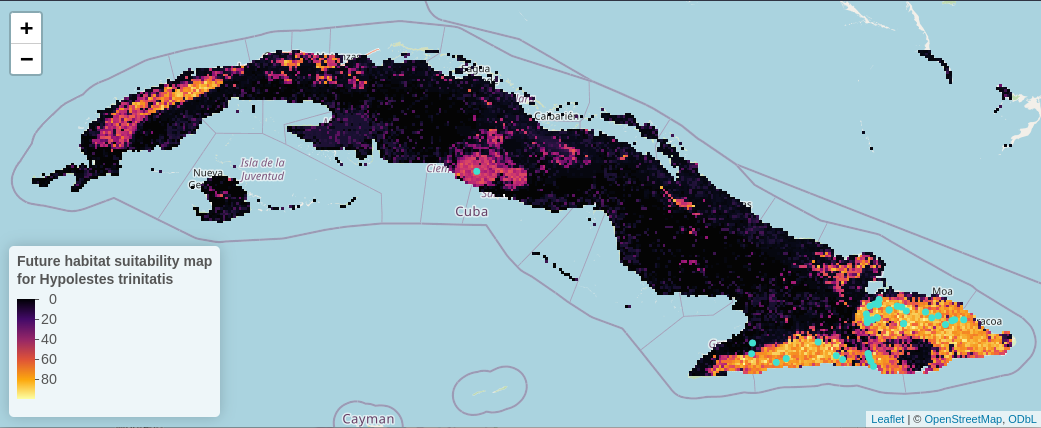

If we zoom in to the habitat suitability map, we can observe the sub-catchments that could offer a suitable habitat to the species in a more detailed view.

References

Amatulli, Giuseppe, Jaime Garcia Marquez, Tushar Sethi, Jens Kiesel, Afroditi Grigoropoulou, Maria M Üblacker, Longzhu Q Shen, and Sami Domisch. 2022. “Hydrography90m: A New High-Resolution Global Hydrographic Dataset.” Earth System Science Data 14 (10): 4525–50.

Appelhans, Tim. 2022. Leafem: Leaflet Extensions for Mapview. https://CRAN.R-project.org/package=leafem.

Appelhans, Tim, Florian Detsch, Christoph Reudenbach, and Stefan Woellauer. 2022. Mapview: Interactive Viewing of Spatial Data in r. https://github.com/r-spatial/mapview.

Cheng, Joe, Barret Schloerke, Bhaskar Karambelkar, and Yihui Xie. 2023. Leaflet: Create Interactive Web Maps with the JavaScript Leaflet Library. https://rstudio.github.io/leaflet/.

Dowle, Matt, and Arun Srinivasan. 2022. Data.table: Extension of ‘Data.frame‘. https://CRAN.R-project.org/package=data.table.

Hijmans, Robert J. 2023. Terra: Spatial Data Analysis. https://rspatial.org/terra/.

Karger, Dirk Nikolaus, and Niklaus E Zimmermann. 2019. “Climatologies at High Resolution for the Earth Land Surface Areas CHELSA V1. 2: Technical Specification.” Swiss Federal Research Institute WSL, Switzerland.

R Core Team. 2022. R: A Language and Environment for Statistical Computing. Vienna, Austria: R Foundation for Statistical Computing. https://www.R-project.org/.

Schürz, Marlene, Afroditi Grigoropoulou, Jaime Garcia Marquez, Yusdiel Torres Cambas, Christoph Schürz, Mathieu Floury, Thomas Tomiczek, Vanessa Bremerich, Giuseppe Amatulli, and Sami Domisch. 2023. Hydrographr: Scalable Hydrographic Data Processing in r. https://glowabio.github.io/hydrographr/.

Torres-Cambas, Yusdiel, Martiño Cabana-Otero, M Olalla Lorenzo-Carballa, and Adolfo Cordero-Rivera. 2016. “Conservation Status and Protection of Three Antillean Endemic Damselflies.” Journal of Insect Conservation 20: 277–84.

Torres-Cambas, Yusdiel, and Juan Carlos Salazar Salina. 2022. “Ephemeroptera, Trichoptera and Odonata of Cuba.” https://doi.org/10.18728/igb-fred-778.3. https://doi.org/10.18728/igb-fred-778.3.

Vaidyanathan, Ramnath, Yihui Xie, JJ Allaire, Joe Cheng, Carson Sievert, and Kenton Russell. 2023. Htmlwidgets: HTML Widgets for r. https://github.com/ramnathv/htmlwidgets.

Valavi, Roozbeh, Jane Elith, José J Lahoz-Monfort, and Gurutzeta Guillera-Arroita. 2021. “Modelling Species Presence-Only Data with Random Forests.” Ecography 44 (12): 1731–42.

Wickham, Hadley. 2022. Stringr: Simple, Consistent Wrappers for Common String Operations. https://CRAN.R-project.org/package=stringr.

Wickham, Hadley, Romain François, Lionel Henry, and Kirill Müller. 2022. Dplyr: A Grammar of Data Manipulation. https://CRAN.R-project.org/package=dplyr.

Wright, Marvin N., Stefan Wager, and Philipp Probst. 2022. Ranger: A Fast Implementation of Random Forests. https://github.com/imbs-hl/ranger.

Wright, Marvin N., and Andreas Ziegler. 2017. “ranger: A Fast Implementation of Random Forests for High Dimensional Data in C++ and R.” Journal of Statistical Software 77 (1): 1–17. https://doi.org/10.18637/jss.v077.i01.

Xie, Yihui. 2014. “Knitr: A Comprehensive Tool for Reproducible Research in R.” In Implementing Reproducible Computational Research, edited by Victoria Stodden, Friedrich Leisch, and Roger D. Peng. Chapman; Hall/CRC.

———. 2015. Dynamic Documents with R and Knitr. 2nd ed. Boca Raton, Florida: Chapman; Hall/CRC. https://yihui.org/knitr/.

———. 2023. Knitr: A General-Purpose Package for Dynamic Report Generation in r. https://yihui.org/knitr/.

Zhu, Hao. 2021. kableExtra: Construct Complex Table with Kable and Pipe Syntax. https://CRAN.R-project.org/package=kableExtra.

Case study - Cuba

Processing of spatial data before and after a Species Distribution Model

2024-01-03